Particle

Here we will describe the particle filter. The state evolves discretely and the measurements are discrete in time. The code is in matlab_implementation/particle. The function header in particle_filter.m is:

function [estimates, covariances] = particle_filter(f_func,jacobian_func,dt_between_measurements,start_time,state_count,sensor_count,measurement_count,particle_count,particle,C,Q_root,R_root,P_0_root,x_0, measurements)

For those familiar with the Kalman filter and notation are familiar with the naming of the variables. However, to be extra sure it is always best to run help particle.

The code is in matlab_implementation/particle of https://github.com/mannyray/KalmanFilter.

We will break down an example below.

Example 1

We will use the same model as in the DD-EKF tab. The example is located in matlab_implementation/particle/examples/logistic2.m and it first runs the code from matlab_implementation/discrete_discrete/examples/logistic.m to define system parameters and then runs the particle filter.

For this example only we can modify matlab_implementation/particle/particle_filter.m by uncommenting the following lines:

%%%particles = cell(measurement_count+1,1);
%%%particles{k} = particle;

and change the function header to have an additional outputs:

function [estimates, covariances, particles] = ...

Now you can run matlab_implementation/particle/examples/logistic2.m:

clear all;
addpath('..');
addpath('../../discrete_discrete');
addpath('../../discrete_discrete/examples');

logistic;
close all;

particle_count = 30; 
pkg load statistics;
particle1 = mvnrnd(x_0-15,P_0,particle_count/2)';
particle2 = mvnrnd(x_0+15,P_0,particle_count/2)';
particle = [particle1,particle2];
[estimates_particle, covariances_particle, particles] = particle_filter(next_func,jacobian_func,dt,t_start,state_count,sensor_count,...
  outputs,particle_count,particle,C,chol(Q_d)',chol(R_d)',chol(P_0)',x_0, measurements);

Now plot the results

h = figure;
hold on;
lim = 975;
plot(0:dt:(outputs-lim-1)*dt,measurements(1:end-lim),'LineWidth',3); 
plot(0:dt:(outputs-lim-1)*dt,process_noise_data(1:end-lim),'LineWidth',3);
plot(0:dt:(outputs-lim-1)*dt,estimates_particle(1:end-lim-1),'LineWidth',3);

for ii=1:(outputs-lim)
    [xUnique, ignore, ixs] = unique(particles{ii});
    counts = zeros(size(xUnique,1),1);
    for ix = 1:size(counts,1);
        counts(ix) = sum(ixs == ix);
    end
    scatter(dt*(ii-1)*ones(length(xUnique),1),xUnique,counts*20,'g','filled');
end
legend('Measurement','Real data','Estimate');
xlabel('Time')
ylabel('Population')

that produces

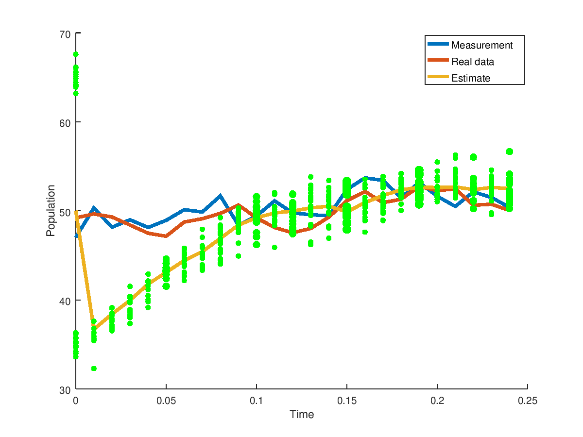
The green dots represent the particles where the thicker dots are where the particles have a higher frequency. The particle filter recovers quickly from the incorrect guess. Don't forget to change back the changes you made in the particle_filter.m code.

Example 2

We will run Example 2 from DD-EKF tab in matlab_implementation/discrete_discrete/examples/linear.m for the particle filter in matlab_implementation/particle/examples/linear2.m or run the code below:

clear all;
addpath('..');
addpath('../../discrete_discrete');
addpath('../../discrete_discrete/examples');

linear;
close all;

particle_count = 30000; 
particle = mvnrnd(x_0,P_0,particle_count)'; 
[estimates_particle, covariances_particle] = particle_filter(func,jacobian_func,dt,t_start,state_count,sensor_count,...
    outputs,particle_count,particle,C,chol(Q_d)',chol(R_d)',chol(P_0)',x_0, measurements);
covariances_particle{end}

to produce

ans =

   5.05404333754918e-07   2.45085320157428e-08
   2.45085320157428e-08   4.98056883303343e-07