Continuous-Discrete Extended Kalman filter

Here we will describe the continuous discrete Extended Kalman filter that is of the square root flavour. Square root does not change the math behind the algorithm, but ensures that numerical rounding errors that are natural to a computer do not prevent the computed covariance matrices maintaining their property of being positive semi definite. For a linear model, the Extended Kalman Filter is equivalent to a regular Kalman filter. Check out this thesis - chapter 3 for a detailed explanation.

For the continuous-discrete Kalman filter the state evolves continuously and the measurements are discrete in time. The code is in matlab_implementation/continuous_discrete of https://github.com/mannyray/KalmanFilter. The estimate is solved for using the RK4. The function header in cdkef.m is:

function [estimates, covariances ] = cdekf(f_func,jacobian_func,dt_between_measurements,rk4_steps, start_time, state_count, sensor_count, measurement_count,C,Q_root,R_root,P_0_root,x_0, measurements)

For those familiar with the Kalman filter and notation are familiar with the naming of the variables. However, to be extra sure it is always best to run help cdekf. We will break down an example below.

Example 1

The example is located in matlab_implementation/continuous_discrete/examples/continuous_logistic.m. You can cd into the directory and then run continuous_logistic or do it step by step as described below. First set the seed and include the path to matlab_implementation/continuous_discrete:

clear all;
addpath('..');

%setting the seed for reproducability
isOctave = exist('OCTAVE_VERSION', 'builtin') ~= 0;
if isOctave==true
    randn("seed",1);
else
    rng(1);
end

Consider the nonlinear continuous logistic growth model. The discrete example can be found in DD-EKF tab.

%define continuous logistic growth model and its jacobian
rate = 0.5; 
max_pop = 100;
deriv_func = @(x) rate*x*(1 - x/max_pop);%logistic population model (quadratic in x)
if isOctave==true
    jacobian_func = @(x) rate - (2*x*rate)/max_pop;%manual derivative - octave might have its own function
else
    %in case you don't want to compute the jacobian manually and you have access
    %to Matlab then you can compute it symbolically and then extract a function from it
    xx = sym('x',[1,1]);
    jacobian_func = matlabFunction(jacobian(deriv_func(xx),xx),'Vars',xx);
end
deriv_func = @(x,t) deriv_func(x) + 0.*t; 
jacobian_func = @(x,t) jacobian_func(x) + 0.*t;

Set the time between each state evolution and the noise covariance and measurement matrices:

%in this model the time is only necessary
%for plotting an interpreting the results.
t_start = 0;
t_final = 10;
outputs = 1000;
dt = (t_final - t_start)/outputs;


R_c = 0.01; 
%discrete noise covariance. 
R_d = 1;
%continuous process noise covariance
Q_c = 10;
%measurement matrix
C = 1;

%generate data and measurements
state_count = 1; 
sensor_count = 1;

Set the initial estimates, covariances as well as generate data in order to run the filter:

%model results if there was no process noise
ideal_data = zeros(state_count,outputs);
%actual data (with process noise) 
process_noise_data = zeros(state_count,outputs);
%noisy measurements of actual data
measurements = zeros(sensor_count,outputs);

%initial condition for ideal
%and real process data
x_0 = max_pop/2;
P_0 = 1;

%initial condition for ideal
%and real process data
x = x_0;
x_noise = x_0;

%generate the data
curTime = t_start;
for ii=1:outputs
    %Explicit Eulers
    x = x + dt.*deriv_func(x,curTime);
    ideal_data(:,ii) = x;

    %Euler-Maruyama
    x_noise = x_noise+dt.*deriv_func(x_noise,curTime)+sqrt(dt.*Q_c)*randn(state_count,1);
    process_noise_data(:,ii) = x_noise;
    measurements(ii) = C*x_noise + sqrt(R_d)*randn(sensor_count,1);

    curTime = curTime + dt;
end

Filter the data:

%filter the noisy measurements
rk4_steps = 1;%internal for code - type 'help cdekf' for more info 
[estimates,covariances] = cdekf(deriv_func,jacobian_func,dt,rk4_steps,t_start,...
    state_count,sensor_count,outputs,C,chol(Q_c)',chol(R_d)',chol(P_0)',x_0,measurements);

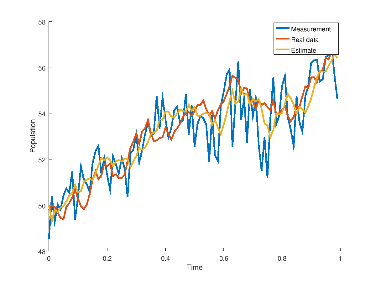
Plot the results:

%The ideal data is not plotted and is only for reference
time = 0:dt:(outputs-1)*dt;
h = figure;
hold on;
limit = 100;
plot(time(1:limit),measurements(1:limit),'LineWidth',2); 
plot(time(1:limit),process_noise_data(1:limit),'LineWidth',2);
plot(time(1:limit),estimates(1:limit),'LineWidth',2);
legend('Measurement','Real data','Estimate');
xlabel('Time')
ylabel('Population')

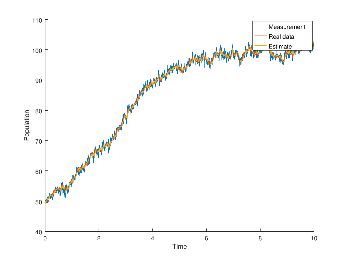
h = figure;
hold on;
plot(0:dt:(outputs-1)*dt,measurements); 
plot(0:dt:(outputs-1)*dt,process_noise_data);
plot(0:dt:(outputs-1)*dt,estimates(1:end-1));
legend('Measurement','Real data','Estimate');
xlabel('Time')
ylabel('Population')

to produce

Example 2

The example is located in matlab_implementation/continuous_discrete/examples/continuous_linear.m and has a model with two states. The script is very similar to the one in the previous example. The result produced is

ans =

   5.0489e-07   2.4509e-08
   2.4509e-08   4.9755e-07