Here we have the Python implementation of discrete discrete Kalman filter (for nonlinear models is the extended Kalman filter). The repository is located at

https://github.com/mannyray/KalmanFilter

The examples here mirror the matlab examples.

Example 1

The example is located in python_implementation/discrete_discrete/examples/logistic.py. You can cd into the directory and then run python logistic.py. We will describe the script here in detail:

import sys
sys.path.insert(0,'..')
from ddekf import *
import numpy as np

Import the ddekf library from the parent directory as well as numpy. Implementation here uses numpy. Next, we set the seed for reproducability:

np.random.seed(1)

Define the nonlinear discrete logistic growth model and its Jacobian function:

rate = 0.01
max_pop = 100.0
def func(x,t):
    return x + rate*x*(1 -(1/max_pop)*x)
def jacobian_func(x,t):
    return 1 + rate - (2*rate/max_pop)*x

For linear functions, the implemenation is equivalent to regular Kalman filter, for nonlinear functions this is the extended Kalman filter. Define the initial estimate x_0, estimate's covariance matrix P_0, process noise matrix Q, sensor noise matrix R and observation matrix C:

x_0 = np.zeros((1,1))
x_0[0][0] = max_pop/2
P_0 = np.array([[1]])
Q = np.array([[1]])
R = np.array([[3]])
C = np.array([[1]])

For accuracy, the implementation of the Kalman filter relies on square root of matrices. We compute the square root matrix:

Q_root = np.linalg.cholesky(Q).transpose()
R_root = np.linalg.cholesky(R).transpose()
P_0_sqrt = np.linalg.cholesky(P_0).transpose()
Q_root = np.array([[1]])

The square root matrix A_sqrt of a matrix A is such that A = A_sqrt.dot(A_sqrt.transpose()). Next, we define our time steps (using start_time, finish_time and dt_between_measurements), the total amount of measurement_count and state_count/sensor_count describes dimensions of the true system state and the measurements:

start_time = 0
finish_time = 10
sensor_count = 1
state_count = 1
measurement_count = 1000
dt_between_measurements = (finish_time - start_time)/measurement_count

Next, we run a simulation where we generate a run of the logistic model and store in process_noise_data (with noise). From process_noise_data, we can generate the noisy measurements and store them in measurements. The process_noise_data will be used later to judge our filter's performance.

x = x_0
x_noise = x_0
ideal_data = []
process_noise_data = []
measurements = []
times = []
for ii in range(0,measurement_count):
    current_time = ii*dt_between_measurements
    times.append(current_time)
    x = func(x,current_time)
    ideal_data.append( x )
    x_noise = func(x_noise,current_time) + Q_root.transpose().dot(np.random.randn(state_count,1))
    process_noise_data.append(x_noise)
    measurements.append(C.dot(x_noise) + R_root.transpose().dot(np.random.randn(sensor_count,1)))

Finally, we use measurements and our previously defined parameteres to run our Kalman filter:

estimates, covariances = ddekf( func, jacobian_func, dt_between_measurements, start_time, state_count, sensor_count, measurement_count, C, Q_root, R_root, P_0_sqrt, x_0, measurements)

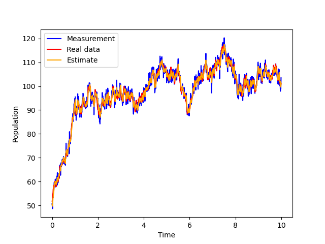
Now we plot the results:

measurements_flat = [ x[0][0] for x in measurements ]
estimates_flat = [ x[0][0] for x in estimates ]
process_noise_data_flat = [ x[0][0] for x in process_noise_data ]
line1, = plt.plot(times,measurements_flat,color='blue',label='Measurement')
line2, = plt.plot(times,process_noise_data_flat,color='red',label='Real data')
line3, = plt.plot(times,estimates_flat[1:],color='orange',label='Estimate')
plt.legend(handles=[line1,line2,line3])
plt.ylabel('Population')
plt.xlabel('Time')
plt.plot()
plt.savefig('logistic2.png')
plt.show()
plt.close()
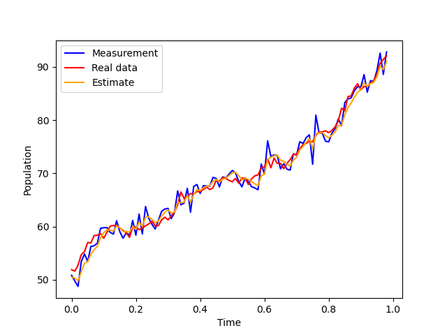
line1, = plt.plot(times[0:99],measurements_flat[0:99],color='blue',label='Measurement')
line2, = plt.plot(times[0:99],process_noise_data_flat[0:99],color='red',label='Real data')
line3, = plt.plot(times[0:99],estimates_flat[1:100],color='orange',label='Estimate')
plt.legend(handles=[line1,line2,line3])
plt.ylabel('Population')
plt.xlabel('Time')
plt.plot()
plt.savefig('logistic1.png')
plt.show()
plt.close()

Example 2

The example is located in python_implementation/discrete_discrete/examples/linear.py and has a model with two states. The result produced is in:

[[5.05404334e-07 2.45085320e-08]

[2.45085320e-08 4.98056883e-07]]