This is a C++ Kalman filter library designed to work with various data types and provide flexibility to use more advanced models. The C++ language may seem verbose to those transitioning from say Python or Matlab. However, this library may seem verbose not only to the Python user but to the C++ user as well. To address this concern, many examples, good documentation and motivation behind the code will be discussed. This is an active project and will continue to grow. I am planning to add additional filters such as the UKF and add further examples. I am looking for help in optimizing the code further as well as adding additional filters and features - if you have ideas, advice or bugs then let me know.
If you are new to Kalman filters then please check out rlabbe's github repository to get an intuition behind the Kalman filter. I assume if you are reading past this point, you have a basic understanding of the Kalman filter, what it requires and common notation used.
First thing let's install the code. The code has been tested on Ubuntu system for now.
The install script only modifies include/Eigen.h. This library is a header-only library.
We will be looking at examples/basicExample.cpp and examples/sampleModel.h in the following tutorial to understand the library. The Kalman filter can be described by the following image (page 147) from Introduction to Random Signals and Applied Kalman Filtering with Matlab Exercises by Robert Grover Brown and Patrick Y. C. Hwang:
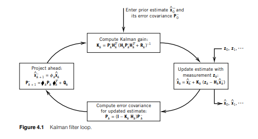
To run this we need a few ingredients. Using the notation from the image, first we need the transition equation for the 'Project ahead' block:
 .
.
In addition, from the 'Project ahead' we need the transition Jacobian  and process noise
  . We need a measurement equation that is not included in the diagram here:
 .
.
Finally, we need the measurement Jacobian  and sensor noise
  . Let's consider a specific system:
![\[ \ddot{x} + \sqrt{2}w_0\dot{x} + w_0^2x = b\sigma u \]](form_6.png)
This ODE describes a damped harmonic oscillator at position  with a forcing white noise term on the right hand side. The equation is taken from
 Introduction to Random Signals and Applied Kalman Filtering with Matlab Exercises section 4.4 Robert Grover Brown and Patrick Y. C. Hwang book mentioned earlier. The model can be expressed as follows
![\[ \frac{d}{dt}\begin{bmatrix}x_1 \\ x_2\end{bmatrix} = \begin{bmatrix} 0 & 1\\ -w_0^2 & -\sqrt{2}w_0 \end{bmatrix} \begin{bmatrix} x_1 \\ x_2 \end{bmatrix} \]](form_8.png)
where  and
and  . Using the Van Loan method described in section 3.9 of the afformentioned source the model can be discretized assuming
  using the following Octave script:
to produce
![\[ \begin{bmatrix} X_1 \\ X_2 \end{bmatrix}_{k+1} = \begin{bmatrix} 0.9952315 & 0.9309552 \\ -0.0093096 & 0.8635746 \end{bmatrix} \begin{bmatrix}X_1 \\ X_2 \end{bmatrix}_k \]](form_12.png)
where  and
and  with process noise
![\[ \bf{Q}_k = \begin{bmatrix} 8.4741e-04 & 1.2257e-03 \\ 1.2257e-03 & 2.4557e-03 \end{bmatrix}. \]](form_15.png)
We will select to measure  only so our measurement equation will be
![\[ z_k = \begin{bmatrix}1 & 0 \end{bmatrix} \begin{bmatrix}X_1 \\ X_2 \end{bmatrix}. \]](form_17.png)
The sensor noise will be
![\[ R_k = (0.5)^2 = 0.25. \]](form_18.png)
The transition jacobian will naturally be
![\[ \begin{bmatrix} 0.9952315 & 0.9309552 \\ -0.0093096 & 0.8635746 \end{bmatrix} \]](form_19.png)
with measurement jacobian
![\[ \begin{bmatrix}1 & 0 \end{bmatrix}. \]](form_20.png)
By now you are familiar with what the Kalman filter needs:
- transition equation
- measurement equation
- process noise covariance
- sensor noise covariance
- transition jacobian
- measurement jacobian
Let's implement the ingredients for our specific example. In this case we will use the Eigen library.
Transition equation
All ingredients or components of a system will inherit from general ingredient or component classes. In this example, we will call the class stateModel and it will inherit from template class discreteModel of Eigen::VectorXd type since we are working with the Eigen library. The general class discreteModel is presented first:
discreteModel is abstract and any class that inherits from it needs to implement the function method. We can use this class to easily implement (1):
stateModel implements function of discreteModel but now has an extra member and even a constructor. This is where the flexibility to the user comes into play. If you want to pass parameters to your constructor in order to have different and multiple instances of a model then you are free to do so. Why have multiple instances? Maybe you are working on tuning your filter or are experimenting with assuming various models. No matter the reason, this library gives you the opportunity to do so easily.
function in this case implements the important relationship of (1). The first argument of function within the Kalman filter will be the previous estimate of the model while time is the current model time which allows for an implementation of a time based model.
Measurement equation
In this instance we implement (2). We will call the class measurementModel:
measurementModel inherits from the same discreteModel class as did stateModel of the transition equation.
Process Noise
discreteModel was used for (1) and (2). Similarly for both sensor and process noise the following base class will be used:
The two pure virtual methods are function and sqrt. function returns the covariance matrix at time t while - the VECTOR input is available for use in case the covariance depends on the state/estimate of the system - such as in distance based applications. The second method is sqrt which will return the Cholesky decomposition (specify which one - upper or lower) which is used for sampling noises in discreteDiscreteFilterSolver (see here for details) and is used in the square root filter.
The process noise (3) is implemented in class processNoise:
In these cases the methods are simple and return an already precomputed result without making use of the arguments as the system is simple. Despite the simplicity, it is the user's responsibility to make sure the dimensions of various matrices, vectors that are returned or used in the various 'ingredients' of the system are logically correct and consistent.
Sensor Noise
### Transition Jacobian
Measurement Jacobian
Putting it all together
Since we have all the ingredients (in examples/sampleModel.h), we are ready to combine them together to define the model. First create instances of the previously discussed classes:
Then specify the state count and sensor count for this specific model
Now we create an instance of the model.
discreteDiscreteFilterModel's purpose is to provide a nice collection of the ingredients in one class while providing an interface layer of the ingredient's methods to other classes. The interface layer allows for easier refactoring of the underlying ingredients.
As probably guessed by the reader, the parameters of discreteDiscreteFilterModel's constructor are pointers to abstract types such as discreteModel which makes the code easy to use for various models/jacobians/noises. The <Eigen::VectorXd,Eigen::MatrixXd> specifies which vector and matrix type is used in the code as the majority of the code is built on templates - read the documentation to make sure the types and function parameters entered are in correct order.
Two classes that depend on the discreteDiscreteFilterModel are discreteDiscreteFilterSolver and the filter itself: discreteDiscreteKalmanFilter. discreteDiscreteFilterSolver is used in cases when one does not have any sample data/measurements and needs to generate them as is common when running simulations. Let's generate some data for our specific model. We need to specify an initial condition and initial time for the system as well:
Let's say we want to solve for 10000 time steps:
To get generated measurements and the true state of the system run:
We now have almost everything. Before running the Kalman filter we need to define our initial estimate and initial covariance:
In our idealized case here the initialEstimate and initialState match up exactly.
If you have read the afformentioned rlabbe repository or studied the Kalman filter previously you will know that the filter consists of the predict and update phase that are repeated for all the measurements over and over again. Hence to filter through the measurements, we run:
We have finally filtered the data and the estimates are stored in estimates array. The user may be wondering why put the burden of running the predict and update on the user and not the Kalman Filter class. Why not simply pass in the measurements array into some method? First of all, if you have gotten all the way here after reviewing the ingridients and are upset with a simple for loop then shame on you. Second of all, the context in which the Kalman filter can be used is diverse. Users may have different output requirements. In addition, passing in a measurement array implies post processing of data and does not allow for 'real time' processing and logic such as adding system input. Finally, it gets the user used to the update/predict terminogy as is common with the Kalman filter and lets them avoid off-by-one logic errors.
Run cd examples; g++ basixExample.cpp; ./a.out to save the data into estimates.txt, states.txt, measurements.txt. We can plot the results using Octave:
to obtain
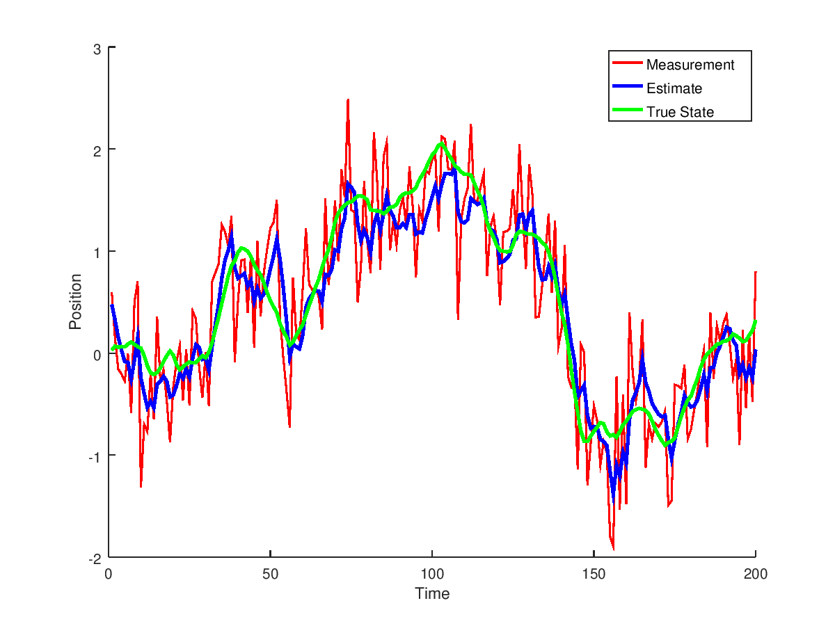
Let's compare the results to the matlab implementation
Testing against the matlab square root implementation
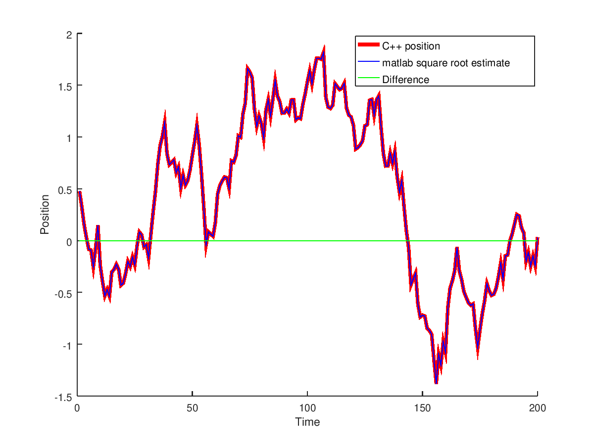
with a maximum error of 1.64246433278281e-04 with max relative error of 56 percent (since they were close to zero estimates with one being 1.56686514969348e-04 while other1.00210021201516e-04). The average relative error is 0.11 percent. The test is passed.
Discussing the templates
Why use templates? The idea is to allow for the use of various matrix/vector libraries in combination with a Kalman filter library. Two main ones that come to mind are Eigen and Boost. The code tutorial above is in examples/basicExample.cpp for the Eigen library while identical boost copy is located within examples/basicExampleBoost.cpp. After compiling and running, the results are identical:
with max difference 3.81361608958741e-14.
examples/basicExamplesBoost.cpp uses a wrapper class from include/mathWrapper that wraps the boost library. The reason for wrapping is because the template class in include/KalmanFitler.h uses operators for matrices and vectors such as + and * that are defined for Eigen but not boost (see 1, 2, 3) or potentially other libraries. In fact, the original example examples/basicExample.cpp uses an extension to the Eigen library in include/Eigen.h instead of the regular <Eigen/Dense> since an additional random vector function needed to be added used in discreteDiscreteFilterSolver. The wrappers will provide the opportunity for further functionality required to implement square root versions of filters.
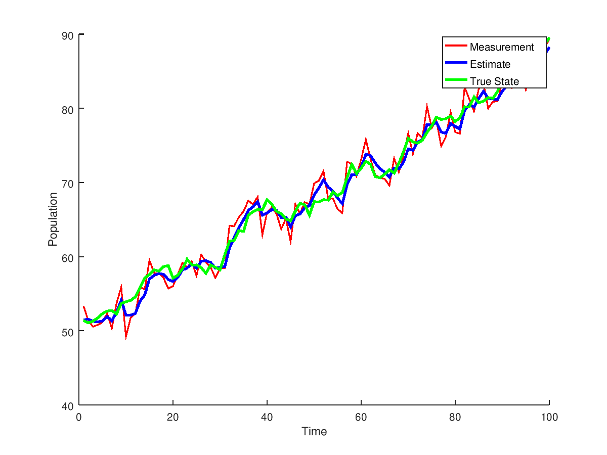
Instead of using Eigen or Boost lets use the good old double to introduce a basic one dimensional nonlinear filtering example.
Nonlinear example:
A nonlinear example is included examples/basicExampleNonlinear.cpp that uses the double wrapper in include/mathWrapper/double.h. This wrapper allows for simple one dimensional examples without needing to install any extra libraries such as Eigen or Boost. The model used is the discrete logistic population growth.